COSMO-LEPS Ensemble Meteograms

The Ensemble Meteogram displays the time evolution of the distribution of selected weather parameters in the COSMO-LEPS ensemble forecasts for a given location. The forecast distribution at each forecast range is represented by a box-and-whiskers plot showing the median (short horizontal line), the 25th and 75th percentiles (wide vertical box), 10th and 90th percentiles (narrower boxes) and the minimum and maximum values (vertical lines).

COSMO-LEPS currently comprises 20 perturbed members, each starting from slightly different initial and boundary conditions (from selected members of ECMWF ENS) plus a deterministic forecast (initial and boundary conditions from ECMWF HRES). COSMO-LEPS runs twice a day, starting at 00 and 12UTC, at the horizontal resolution of 7km, 40 model levels in the vertical and a forecast range of 132 hours.

When creating COSMO-LEPS Meteograms, the nearest land point is selected, or if only sea points are available, the nearest one of those is used; this situation is noted in the Meteogram's title section with the words "EPS sea point". The Meteograms provide forecast distributions at 6-hour intervals up to 132 hours for the following parameters:

Total cloud cover

instantaneous forecast value, in oktas (eighths of the sky covered by cloud).

Total precipitation

accumulated precipitation (sum of convective and large scale) over the six hour period preceding the x-axis time, in mm. A scaling is sometimes applied to the precipitation Y-axis to avoid the undesirable effect of large extreme values stretching the scale so much that the information on smaller amounts cannot be resolved. The largest 6-hourly maxima are shown at the top as red numbers if this scaling is used.

10m wind speed

instantaneous forecast (mean) value, in m/s.

2m temperature

instantaneous forecast value, in degrees Celsius (^oC). The model orography can differ significantly from the station height, which necessitates some temperature correction. The forecast temperature is adjusted by 6.5 ^oC per 1000 metres difference between the station height and the model orography. Note that in the case of temperature inversions the forecast of 2m temperature needs to be used with great care.

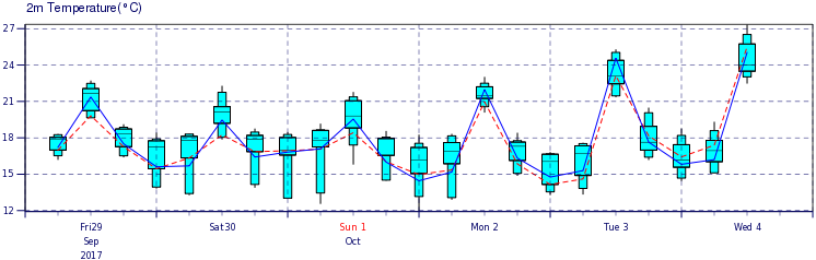
The single deterministic forecast is also shown, using a     red dashed line